One recurring frustration that I have with Matplotlib is how the pcolor and pcolormesh functions work. (I tend to use pcolormesh more, since the two functions are practically the same but the latter much faster.)
You may be familiar with them: given a set of x,y, and z values, pcolor and pcolormesh plot individual data as filled pixels corresponding to a color map range you specify. Here’s an example using the NCAR Large Ensemble’s topography file (download it here).
First, import necessary Python packages and open the topography file:
import xarray
import cartopy
import numpy as np
import matplotlib.pyplot as plt
topo_file = xarray.open_dataset('USGS-gtopo30_0.9x1.25_remap_c051027.nc')
Printing topo_file to screen gives this:
>>> print(topo_file)

<xarray.Dataset>
Dimensions:       (lat: 192, lon: 288)
Coordinates:
  * lat           (lat) float64 -90.0 -89.06 -88.12 -87.17 -86.23 -85.29 ...
  * lon           (lon) float64 0.0 1.25 2.5 3.75 5.0 6.25 7.5 8.75 10.0 ...
Data variables:
    PHIS          (lat, lon) float64 2.77e+04 2.77e+04 2.77e+04 2.77e+04 ...
    SGH           (lat, lon) float64 ...
    SGH30         (lat, lon) float64 ...
    LANDFRAC      (lat, lon) float64 1.0 1.0 1.0 1.0 1.0 1.0 1.0 1.0 1.0 1.0 ...
    LANDM_COSLAT  (lat, lon) float64 ...
Attributes:
    history:    Written on date: 20051027\ndefinesurf -remap -t /fs/cgd/csm/i...
    make_ross:  true
    topofile:   /fs/cgd/csm/inputdata/atm/cam/topo/USGS-gtopo30_10min_c050419.nc
    gridfile:   /fs/cgd/csm/inputdata/atm/cam/coords/fv_0.9x1.25.nc
    landmask:   /fs/cgd/csm/inputdata/atm/cam2/hrtopo/landm_coslat.nc
Note the field we want is PHIS, which is the surface geopotential. If the NetCDF file has metadata with it, you can interrogate the units by printing the specific variable:
>>> print(topo_file['PHIS'])

<xarray.DataArray 'PHIS' (lat: 192, lon: 288)>
array([[27701.627574, 27701.627574, 27701.627574, ..., 27701.627574,
        27701.627574, 27701.627574],
       [26781.993496, 26801.877955, 26823.24702 , ..., 26731.480458,
        26746.794726, 26763.628318],
       [25888.717611, 25951.505898, 26014.836766, ..., 25705.620241,
        25765.581423, 25826.676211],
       ...,
       [    0.      ,     0.      ,     0.      , ...,     0.      ,
            0.      ,     0.      ],
       [    0.      ,     0.      ,     0.      , ...,     0.      ,
            0.      ,     0.      ],
       [    0.      ,     0.      ,     0.      , ...,     0.      ,
            0.      ,     0.      ]])
Coordinates:
  * lat      (lat) float64 -90.0 -89.06 -88.12 -87.17 -86.23 -85.29 -84.35 ...
  * lon      (lon) float64 0.0 1.25 2.5 3.75 5.0 6.25 7.5 8.75 10.0 11.25 ...
Attributes:
    long_name:   surface geopotential
    units:       m2/s2
    from_hires:  true
    filter:      remap
Looks like the units attribute tells us this field is m2s-2. Divide by gravitational acceleration (9.81) to get back meters. This will be our z value in pcolormesh:
topo_data = topo_file['PHIS'].values/9.81 # surf geopot. divided by gravity
Also pull out the land fraction values and set everything <0.1 (i.e., less than 10% land) to a np.nan (NaN value in Numpy). I do this kind of thing when I want to apply an ocean mask, for example:
landfrac_data = topo_file['LANDFRAC'].values
topo_data[landfrac_data==0]=np.nan
Finally, grab the longitude and latitude arrays, which will serve as our x and y values:
lon = topo_file['lon'].values
lat = topo_file['lat'].values
contourf looks fine…
Now let’s plot topography for a given region—I’ve chosen Indonesia here, because it illustrates the problem well. Using contourf, you can code up something like this:
map_proj = cartopy.crs.PlateCarree()
data_proj = cartopy.crs.PlateCarree()
geodetic_proj = cartopy.crs.PlateCarree()

fig = plt.figure(figsize=(5,3.25))

ax = fig.add_subplot(111, projection=map_proj)
ax.coastlines()

topo_plot = ax.contourf(lon,\
                        lat,\
                        topo_data,\
                        levels=[0,200,400,600,800,1000],\
                        extend='max',\
                        transform=data_proj)
ax.set_extent([90,160,-20,20])

# add colorbar
axpos = ax.get_position()
cbar_ax = fig.add_axes([axpos.x1+0,axpos.y0,0.03,axpos.height])
cbar = fig.colorbar(topo_plot, cax=cbar_ax)
cbar.ax.tick_params(labelsize=12)
cbar.set_label('elevation (m)', fontsize=12)
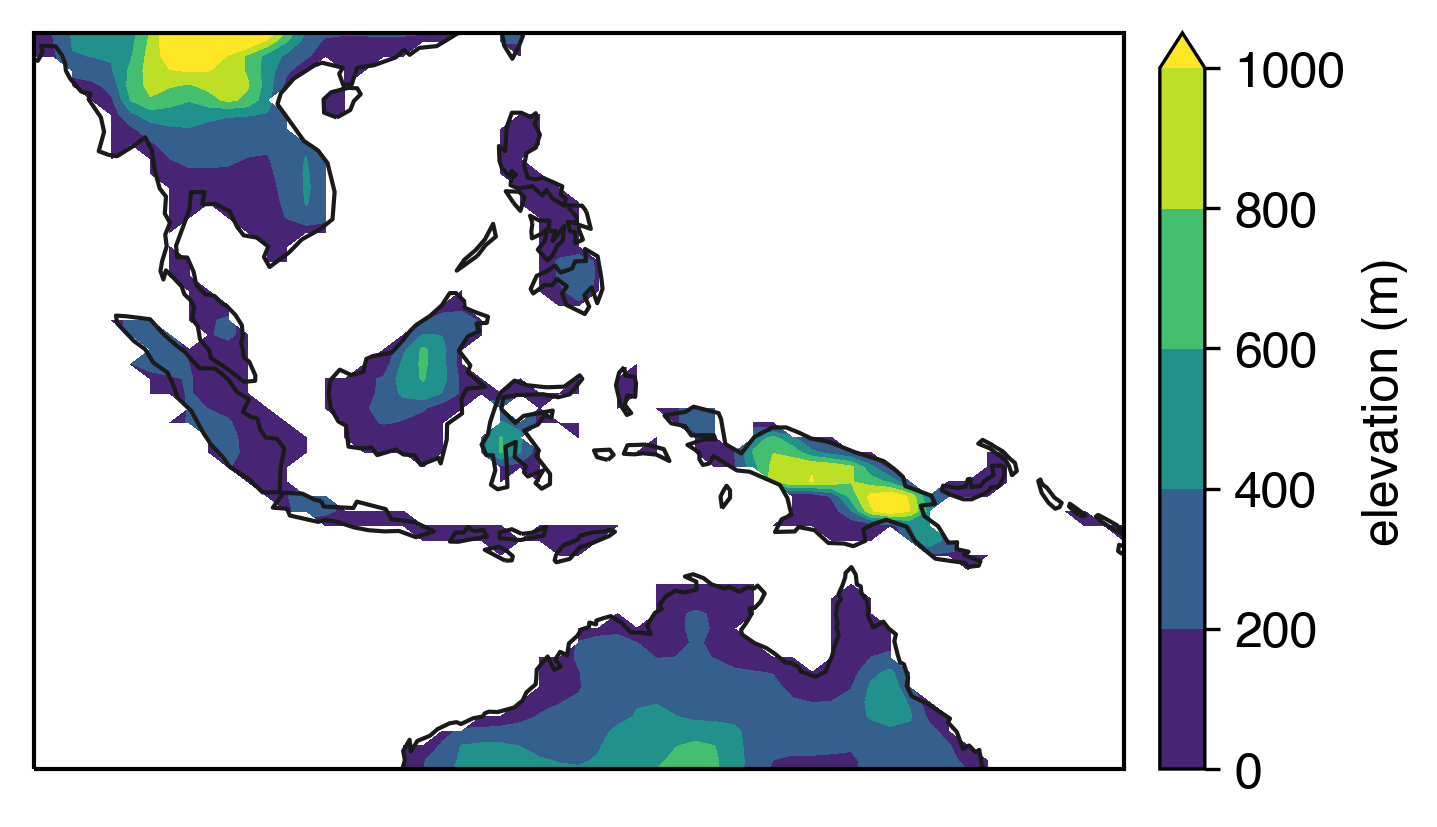
Notice the edges are a little rough looking, since contourf is interpolating up against NaN values that we placed into the data array where there was less than 10% land.
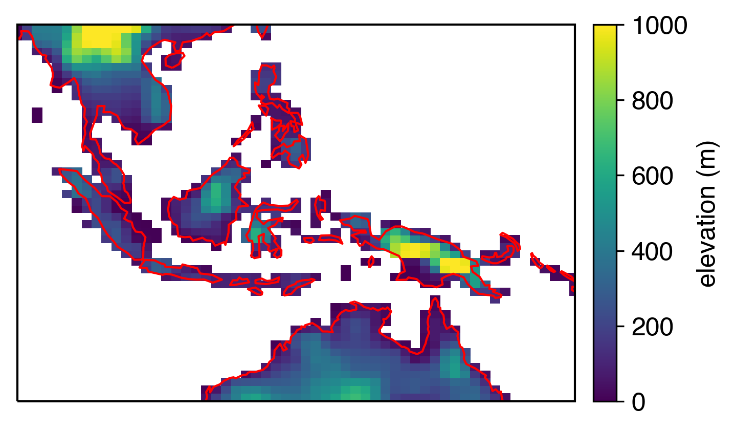
…but pcolormesh is offset
If we plot the same thing in pcolormesh, the pixels represent the model resolution directly, which can be a nice bit of information to add to the figure. But this is where it gets annoying: the coastlines are offset from the grid. It’s pretty obvious if we plot them in red; notice a southwestern offset:
map_proj = cartopy.crs.PlateCarree()
data_proj = cartopy.crs.PlateCarree()
geodetic_proj = cartopy.crs.PlateCarree()

fig = plt.figure(figsize=(5,3.25))

ax = fig.add_subplot(111, projection=map_proj)
ax.coastlines(color='red')

topo_plot = ax.pcolormesh(lon,\
                          lat,\
                          topo_data,vmin=0,vmax=1000,\
                          transform=data_proj)
ax.set_extent([90,160,-20,20])

# add colorbar
axpos = ax.get_position()
cbar_ax = fig.add_axes([axpos.x1+0,axpos.y0,0.03,axpos.height])
cbar = fig.colorbar(topo_plot, cax=cbar_ax)
cbar.ax.tick_params(labelsize=12)
cbar.set_label('elevation (m)', fontsize=12)

I realize that this kind of thing isn’t that bad, especially if you’re looking at global plots where coastline details matter less. But I avoided pcolormesh for a long time because of this effect. When you zoom in, it looks even worse:
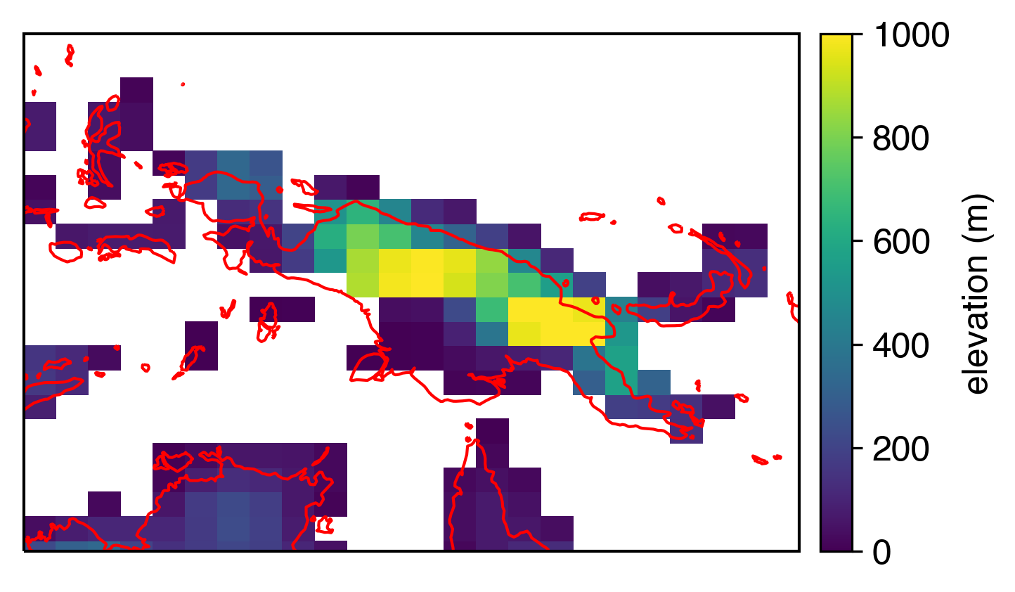
Gross.
So what’s going on? That can be found in the pcolor documentation: There’s actually an interpolation happening, where the function interpolates the original grid to its vertices and thereby shortens the latitude and longitude data by a row and column each. So the elevation values plotted above are correct; there’s no interpolation happening there (to my knowledge). It’s just that the latitude and longitude grids have been interpolated internally, leading to the offset seen relative to the map.
Fix it by interpolating latitude and longitude arrays to midpoints
As far as I know, there’s no keyword or True/False switch in pcolormesh to fix this. Instead, you need to feed it a shifted grid that it will internally interpolate. To do this, my approach is to:
- Add two rows and columns to the latitude and longitude grids (one on each side)
- Interpolate to the center of those values and feed them into
pcolormesh, so that its own interpolation creates the original grid
Here’s an example; note this works best on regular, equally-spaced grids (the kind that CMIP models typically use in standard output), but if they’re irregular it will still probably be better than doing nothing…
# extend longitude by 2
lon_extend = np.zeros(lon.size+2)
# fill in internal values
lon_extend[1:-1] = lon # fill up with original values
# fill in extra endpoints
lon_extend[0] = lon[0]-np.diff(lon)[0]
lon_extend[-1] = lon[-1]+np.diff(lon)[-1]
# calculate the midpoints
lon_pcolormesh_midpoints = lon_extend[:-1]+0.5*(np.diff(lon_extend))

# extend latitude by 2
lat_extend = np.zeros(lat.size+2)
# fill in internal values
lat_extend[1:-1] = lat
# fill in extra endpoints
lat_extend[0] = lat[0]-np.diff(lat)[0]
lat_extend[-1] = lat[-1]+np.diff(lat)[-1]
# calculate the midpoints
lat_pcolormesh_midpoints = lat_extend[:-1]+0.5*(np.diff(lat_extend))
The above code isn’t very complicated, and I imagine it can be simplified a lot more. For example, I use np.diff() to calculate the spacing between latitude and longitude points. If all of your values are equally spaced, you can just use the actual step value here (e.g., for a 2.5x2.5º grid, use 2.5 as the spacing). To be safer, though, I use the diff function, which I do in case the grid is not regularly spaced.
Now plug in the lon_pcolormesh_midpoints and lat_pcolormesh_midpoints arrays as your new x and y values. The size of each is one longer than the dimensions of the original topo_data.
map_proj = cartopy.crs.PlateCarree()
data_proj = cartopy.crs.PlateCarree()
geodetic_proj = cartopy.crs.PlateCarree()

fig = plt.figure(figsize=(5,3.25))

ax = fig.add_subplot(111, projection=map_proj)
ax.coastlines(color='red')

topo_plot = ax.pcolormesh(lon_pcolormesh_midpoints,\
                          lat_pcolormesh_midpoints,\
                          topo_data,vmin=0,vmax=1000,\
                          transform=data_proj)
ax.set_extent([90,160,-20,20])

# add colorbar
axpos = ax.get_position()
cbar_ax = fig.add_axes([axpos.x1+0,axpos.y0,0.03,axpos.height])
cbar = fig.colorbar(topo_plot, cax=cbar_ax)
cbar.ax.tick_params(labelsize=12)
cbar.set_label('elevation (m)', fontsize=12)
Now it’s looking good…
…even when we zoom in:
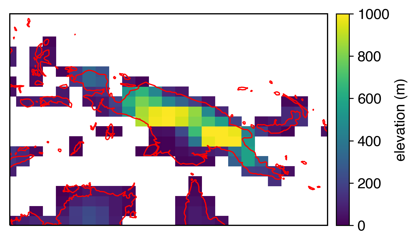
The coarseness of the model grid is still going to look a little funny against coastlines, but that’s about as good as we can get at this resolution (which is about 1x1º).
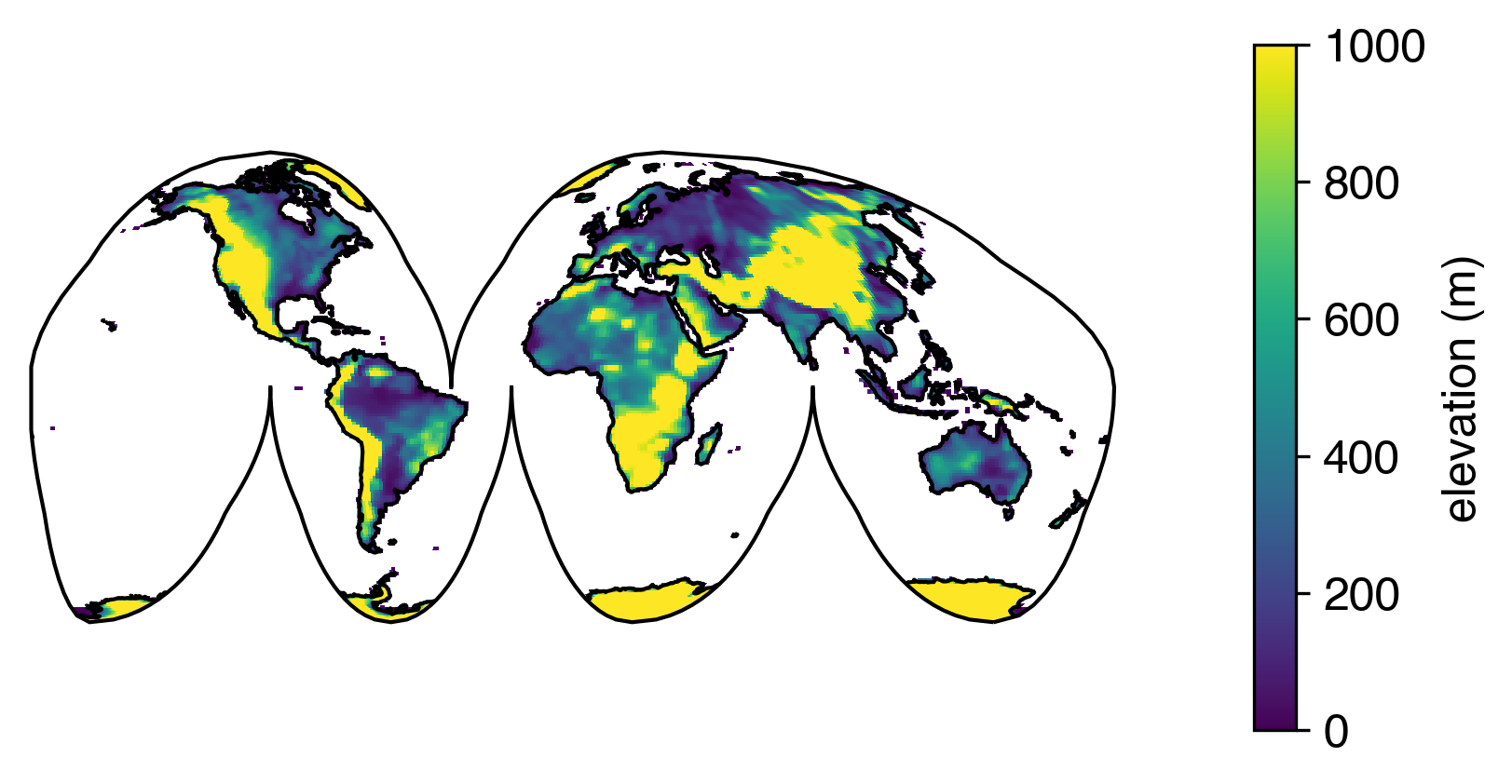
Even on a global grid that requires reprojection, with this fix to pcolormesh, we can be rest-assured that the coastlines are lining up as well as they can:
What if latitude and longitude are two-dimensional arrays?
This should be pretty easy—you’ll just need to be a little fancier with the array subsetting when calculating the midpoints.
Something like this should work (but I haven’t tested it enough, so it’s not once-size-fits-all):
# extend longitude by 2
lon_extend = np.zeros(lon.shape[0],lon.shape[1]+2)
# fill in internal values
lon_extend[:,1:-1] = lon # fill up with original values
# fill in extra endpoints
lon_extend[:,0] = lon[:,0]-np.diff(lon, axis=1)
lon_extend[:,-1] = lon[:,-1]+np.diff(lon, axis=1)
# calculate the midpoints
lon_pcolormesh_midpoints = lon_extend[:,:-1]+0.5*(np.diff(lon_extend, axis=1))

# extend latitude by 2
lat_extend = np.zeros(lat.shape[0]+2,lat.shape[1])
# fill in internal values
lat_extend[1:-1,:] = lat
# fill in extra endpoints
lat_extend[0,:] = lat[0,:]-np.diff(lat, axis=0)
lat_extend[-1,:] = lat[-1,:]+np.diff(lat, axis=0)
# calculate the midpoints
lat_pcolormesh_midpoints = lat_extend[:-1,:]+0.5*(np.diff(lat_extend, axis=0))